import pandas as pd
import numpy as np
import matplotlib.pyplot as plt
from datetime import datetime
from datetime import timedelta
from pandas.plotting import register_matplotlib_converters
from statsmodels.tsa.stattools import acf, pacf
from statsmodels.tsa.statespace.sarimax import SARIMAX
register_matplotlib_converters()
from time import time
11: Anomaly Detection#
def parser(s):
    return datetime.strptime(s, '%Y-%m-%d')
#read data
catfish_sales = pd.read_csv('../data/catfish.csv', parse_dates=[0], index_col=0, squeeze=True, date_parser=parser)
/tmp/ipykernel_3777558/2935818357.py:2: FutureWarning: The squeeze argument has been deprecated and will be removed in a future version. Append .squeeze("columns") to the call to squeeze.


  catfish_sales = pd.read_csv('../data/catfish.csv', parse_dates=[0], index_col=0, squeeze=True, date_parser=parser)
#infer the frequency of the data
catfish_sales = catfish_sales.asfreq(pd.infer_freq(catfish_sales.index))
start_date = datetime(1996,1,1)
end_date = datetime(2000,1,1)
lim_catfish_sales = catfish_sales[start_date:end_date]
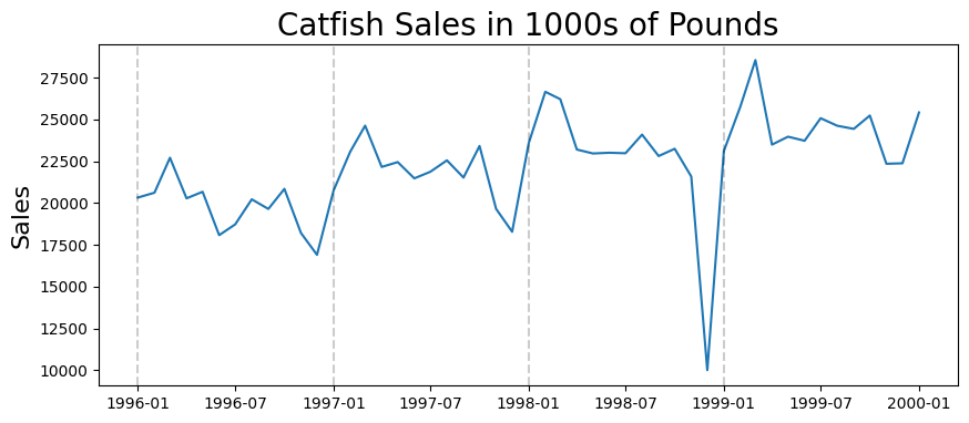
#At December 1 1998
lim_catfish_sales[datetime(1998,12,1)] = 10000
plt.figure(figsize=(10,4))
plt.plot(lim_catfish_sales)
plt.title('Catfish Sales in 1000s of Pounds', fontsize=20)
plt.ylabel('Sales', fontsize=16)
for year in range(start_date.year,end_date.year):
    plt.axvline(pd.to_datetime(str(year)+'-01-01'), color='k', linestyle='--', alpha=0.2)
Remove the trend#
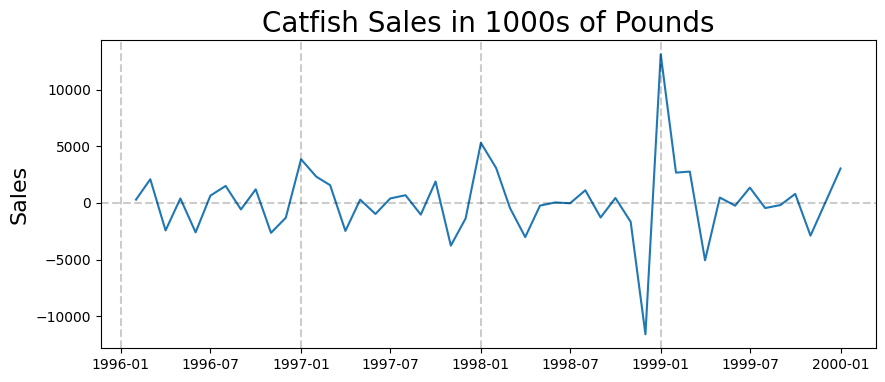
first_diff = lim_catfish_sales.diff()[1:]
plt.figure(figsize=(10,4))
plt.plot(first_diff)
plt.title('Catfish Sales in 1000s of Pounds', fontsize=20)
plt.ylabel('Sales', fontsize=16)
for year in range(start_date.year,end_date.year):
    plt.axvline(pd.to_datetime(str(year)+'-01-01'), color='k', linestyle='--', alpha=0.2)
plt.axhline(0, color='k', linestyle='--', alpha=0.2)
<matplotlib.lines.Line2D at 0x7f10b1cedca0>
Get training and testing sets#
train_end = datetime(1999,7,1)
test_end = datetime(2000,1,1)

test_data = lim_catfish_sales[train_end + timedelta(days=1):test_end]
Make Predictions#
my_order = (0,1,0)
my_seasonal_order = (1, 0, 1, 12)
rolling_predictions = test_data.copy()
for train_end in test_data.index:
    train_data = lim_catfish_sales[:train_end-timedelta(days=1)]
    model = SARIMAX(train_data, order=my_order, seasonal_order=my_seasonal_order)
    model_fit = model.fit()

    pred = model_fit.forecast()
    rolling_predictions[train_end] = pred
/home/ubuntu/Documents/Projects/STI_FX_Intervention/.venv/lib/python3.9/site-packages/statsmodels/tsa/statespace/sarimax.py:997: UserWarning: Non-stationary starting seasonal autoregressive Using zeros as starting parameters.
  warn('Non-stationary starting seasonal autoregressive'
/home/ubuntu/Documents/Projects/STI_FX_Intervention/.venv/lib/python3.9/site-packages/statsmodels/tsa/statespace/sarimax.py:1009: UserWarning: Non-invertible starting seasonal moving average Using zeros as starting parameters.
  warn('Non-invertible starting seasonal moving average'
 This problem is unconstrained.
RUNNING THE L-BFGS-B CODE

           * * *

Machine precision = 2.220D-16
 N =            3     M =           10

At X0         0 variables are exactly at the bounds

At iterate    0    f=  1.00865D+01    |proj g|=  1.88677D+00

At iterate    5    f=  9.42806D+00    |proj g|=  1.15193D-01

At iterate   10    f=  9.37825D+00    |proj g|=  3.57802D-03

At iterate   15    f=  9.37017D+00    |proj g|=  1.52764D-02

At iterate   20    f=  9.25763D+00    |proj g|=  1.18506D-01

At iterate   25    f=  9.21700D+00    |proj g|=  9.28828D-04

           * * *

Tit   = total number of iterations
Tnf   = total number of function evaluations
Tnint = total number of segments explored during Cauchy searches
Skip  = number of BFGS updates skipped
Nact  = number of active bounds at final generalized Cauchy point
Projg = norm of the final projected gradient
F     = final function value

           * * *

   N    Tit     Tnf  Tnint  Skip  Nact     Projg        F
    3     27     29      1     0     0   9.042D-08   9.217D+00
  F =   9.2169957488805672

CONVERGENCE: NORM_OF_PROJECTED_GRADIENT_<=_PGTOL
/home/ubuntu/Documents/Projects/STI_FX_Intervention/.venv/lib/python3.9/site-packages/statsmodels/tsa/statespace/sarimax.py:1009: UserWarning: Non-invertible starting seasonal moving average Using zeros as starting parameters.
  warn('Non-invertible starting seasonal moving average'
 This problem is unconstrained.
RUNNING THE L-BFGS-B CODE

           * * *

Machine precision = 2.220D-16
 N =            3     M =           10

At X0         0 variables are exactly at the bounds

At iterate    0    f=  1.08193D+01    |proj g|=  5.52980D-01

At iterate    5    f=  9.46761D+00    |proj g|=  9.12352D-02

At iterate   10    f=  9.40117D+00    |proj g|=  4.02561D-02

At iterate   15    f=  9.36519D+00    |proj g|=  2.66287D-02
  ys=-2.680E-02  -gs= 6.684E-03 BFGS update SKIPPED
  ys=-3.133E-06  -gs= 2.118E-07 BFGS update SKIPPED
 Bad direction in the line search;
   refresh the lbfgs memory and restart the iteration.
At iterate   20    f=  9.35244D+00    |proj g|=  6.45941D-03

At iterate   25    f=  9.35242D+00    |proj g|=  5.26224D-03
 Bad direction in the line search;
   refresh the lbfgs memory and restart the iteration.

 Bad direction in the line search;
   refresh the lbfgs memory and restart the iteration.
At iterate   30    f=  9.35237D+00    |proj g|=  7.37719D-03

At iterate   35    f=  9.35225D+00    |proj g|=  1.23386D-02
  ys=-1.927E-04  -gs= 3.436E-05 BFGS update SKIPPED

At iterate   40    f=  9.35219D+00    |proj g|=  1.73730D-02
  ys=-2.328E-07  -gs= 1.077E-07 BFGS update SKIPPED
 Bad direction in the line search;
   refresh the lbfgs memory and restart the iteration.

 Warning:  more than 10 function and gradient
   evaluations in the last line search.  Termination
   may possibly be caused by a bad search direction.
/home/ubuntu/Documents/Projects/STI_FX_Intervention/.venv/lib/python3.9/site-packages/statsmodels/tsa/statespace/sarimax.py:997: UserWarning: Non-stationary starting seasonal autoregressive Using zeros as starting parameters.
  warn('Non-stationary starting seasonal autoregressive'
/home/ubuntu/Documents/Projects/STI_FX_Intervention/.venv/lib/python3.9/site-packages/statsmodels/tsa/statespace/sarimax.py:1009: UserWarning: Non-invertible starting seasonal moving average Using zeros as starting parameters.
  warn('Non-invertible starting seasonal moving average'
 This problem is unconstrained.
At iterate   45    f=  9.35217D+00    |proj g|=  1.62073D-03

           * * *

Tit   = total number of iterations
Tnf   = total number of function evaluations
Tnint = total number of segments explored during Cauchy searches
Skip  = number of BFGS updates skipped
Nact  = number of active bounds at final generalized Cauchy point
Projg = norm of the final projected gradient
F     = final function value

           * * *

   N    Tit     Tnf  Tnint  Skip  Nact     Projg        F
    3     45    228      5     4     0   1.621D-03   9.352D+00
  F =   9.3521737365165123

CONVERGENCE: REL_REDUCTION_OF_F_<=_FACTR*EPSMCH
RUNNING THE L-BFGS-B CODE

           * * *

Machine precision = 2.220D-16
 N =            3     M =           10

At X0         0 variables are exactly at the bounds

At iterate    0    f=  1.02169D+01    |proj g|=  2.05161D+00

At iterate    5    f=  9.45797D+00    |proj g|=  6.72771D-02

At iterate   10    f=  9.40808D+00    |proj g|=  2.42390D-03

At iterate   15    f=  9.39350D+00    |proj g|=  2.13080D-02

At iterate   20    f=  9.20360D+00    |proj g|=  1.32847D-02

At iterate   25    f=  9.20276D+00    |proj g|=  2.92847D-05

           * * *

Tit   = total number of iterations
Tnf   = total number of function evaluations
Tnint = total number of segments explored during Cauchy searches
Skip  = number of BFGS updates skipped
Nact  = number of active bounds at final generalized Cauchy point
Projg = norm of the final projected gradient
F     = final function value

           * * *

   N    Tit     Tnf  Tnint  Skip  Nact     Projg        F
    3     26     29      1     0     0   2.867D-05   9.203D+00
  F =   9.2027590959410581

CONVERGENCE: REL_REDUCTION_OF_F_<=_FACTR*EPSMCH
/home/ubuntu/Documents/Projects/STI_FX_Intervention/.venv/lib/python3.9/site-packages/statsmodels/tsa/statespace/sarimax.py:1009: UserWarning: Non-invertible starting seasonal moving average Using zeros as starting parameters.
  warn('Non-invertible starting seasonal moving average'
 This problem is unconstrained.

 Warning:  more than 10 function and gradient
   evaluations in the last line search.  Termination
   may possibly be caused by a bad search direction.
RUNNING THE L-BFGS-B CODE

           * * *

Machine precision = 2.220D-16
 N =            3     M =           10

At X0         0 variables are exactly at the bounds

At iterate    0    f=  9.74977D+00    |proj g|=  6.76205D-01

At iterate    5    f=  9.42227D+00    |proj g|=  3.14046D-01

At iterate   10    f=  9.24662D+00    |proj g|=  7.58416D-02

At iterate   15    f=  9.20068D+00    |proj g|=  2.17069D-02

At iterate   20    f=  9.17745D+00    |proj g|=  5.55019D-02
  ys=-1.070E-01  -gs= 1.840E-02 BFGS update SKIPPED

           * * *

Tit   = total number of iterations
Tnf   = total number of function evaluations
Tnint = total number of segments explored during Cauchy searches
Skip  = number of BFGS updates skipped
Nact  = number of active bounds at final generalized Cauchy point
Projg = norm of the final projected gradient
F     = final function value

           * * *

   N    Tit     Tnf  Tnint  Skip  Nact     Projg        F
    3     21     41      1     1     0   5.597D-02   9.177D+00
  F =   9.1774487580915114

CONVERGENCE: REL_REDUCTION_OF_F_<=_FACTR*EPSMCH
/home/ubuntu/Documents/Projects/STI_FX_Intervention/.venv/lib/python3.9/site-packages/statsmodels/tsa/statespace/sarimax.py:1009: UserWarning: Non-invertible starting seasonal moving average Using zeros as starting parameters.
  warn('Non-invertible starting seasonal moving average'
 This problem is unconstrained.
RUNNING THE L-BFGS-B CODE

           * * *

Machine precision = 2.220D-16
 N =            3     M =           10

At X0         0 variables are exactly at the bounds

At iterate    0    f=  1.06607D+01    |proj g|=  5.90030D-01

At iterate    5    f=  9.41178D+00    |proj g|=  1.06608D-01

At iterate   10    f=  9.34059D+00    |proj g|=  4.62385D-02

At iterate   15    f=  9.30427D+00    |proj g|=  5.71632D-02
  ys=-1.872E-01  -gs= 1.328E-02 BFGS update SKIPPED
 Bad direction in the line search;
   refresh the lbfgs memory and restart the iteration.
/home/ubuntu/Documents/Projects/STI_FX_Intervention/.venv/lib/python3.9/site-packages/statsmodels/tsa/statespace/sarimax.py:1009: UserWarning: Non-invertible starting seasonal moving average Using zeros as starting parameters.
  warn('Non-invertible starting seasonal moving average'
 This problem is unconstrained.
At iterate   20    f=  9.29452D+00    |proj g|=  4.89056D-03

           * * *

Tit   = total number of iterations
Tnf   = total number of function evaluations
Tnint = total number of segments explored during Cauchy searches
Skip  = number of BFGS updates skipped
Nact  = number of active bounds at final generalized Cauchy point
Projg = norm of the final projected gradient
F     = final function value

           * * *

   N    Tit     Tnf  Tnint  Skip  Nact     Projg        F
    3     21     72      2     1     0   5.177D-03   9.295D+00
  F =   9.2945184761749271

CONVERGENCE: REL_REDUCTION_OF_F_<=_FACTR*EPSMCH
RUNNING THE L-BFGS-B CODE

           * * *

Machine precision = 2.220D-16
 N =            3     M =           10

At X0         0 variables are exactly at the bounds

At iterate    0    f=  9.44886D+00    |proj g|=  6.73274D-01

At iterate    5    f=  9.32563D+00    |proj g|=  5.75231D-01

At iterate   10    f=  9.10124D+00    |proj g|=  7.51289D-02

At iterate   15    f=  9.05847D+00    |proj g|=  1.32918D-02

At iterate   20    f=  9.04952D+00    |proj g|=  9.02023D-03

At iterate   25    f=  9.04658D+00    |proj g|=  1.69952D-03

At iterate   30    f=  9.04650D+00    |proj g|=  5.39719D-04

           * * *

Tit   = total number of iterations
Tnf   = total number of function evaluations
Tnint = total number of segments explored during Cauchy searches
Skip  = number of BFGS updates skipped
Nact  = number of active bounds at final generalized Cauchy point
Projg = norm of the final projected gradient
F     = final function value

           * * *

   N    Tit     Tnf  Tnint  Skip  Nact     Projg        F
    3     32     49      1     0     0   5.630D-03   9.046D+00
  F =   9.0464650017000530

CONVERGENCE: REL_REDUCTION_OF_F_<=_FACTR*EPSMCH
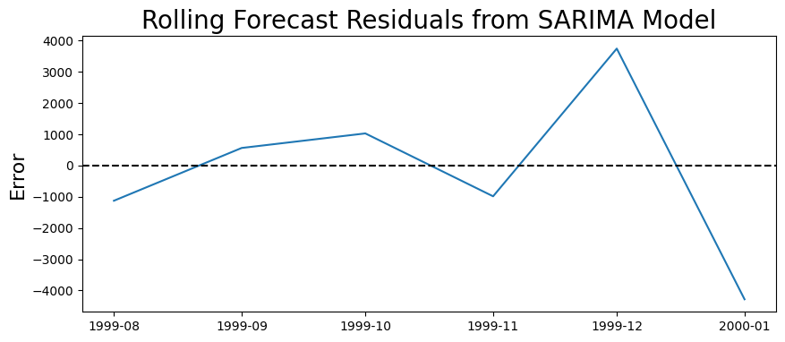
rolling_residuals = test_data - rolling_predictions
plt.figure(figsize=(10,4))
plt.plot(rolling_residuals)
plt.axhline(0, linestyle='--', color='k')
plt.title('Rolling Forecast Residuals from SARIMA Model', fontsize=20)
plt.ylabel('Error', fontsize=16)
Text(0, 0.5, 'Error')
plt.figure(figsize=(10,4))

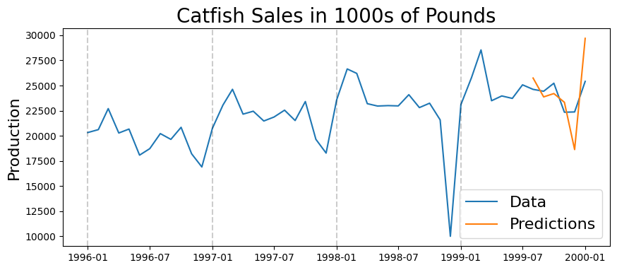
plt.plot(lim_catfish_sales)
plt.plot(rolling_predictions)

plt.legend(('Data', 'Predictions'), fontsize=16)

plt.title('Catfish Sales in 1000s of Pounds', fontsize=20)
plt.ylabel('Production', fontsize=16)
for year in range(start_date.year,end_date.year):
    plt.axvline(pd.to_datetime(str(year)+'-01-01'), color='k', linestyle='--', alpha=0.2)
print('Mean Absolute Percent Error:', round(np.mean(abs(rolling_residuals/test_data)),4))
Mean Absolute Percent Error: 0.0815
print('Root Mean Squared Error:', np.sqrt(np.mean(rolling_residuals**2)))
Root Mean Squared Error: 2447.4759538453186
Detecting the Anomaly#
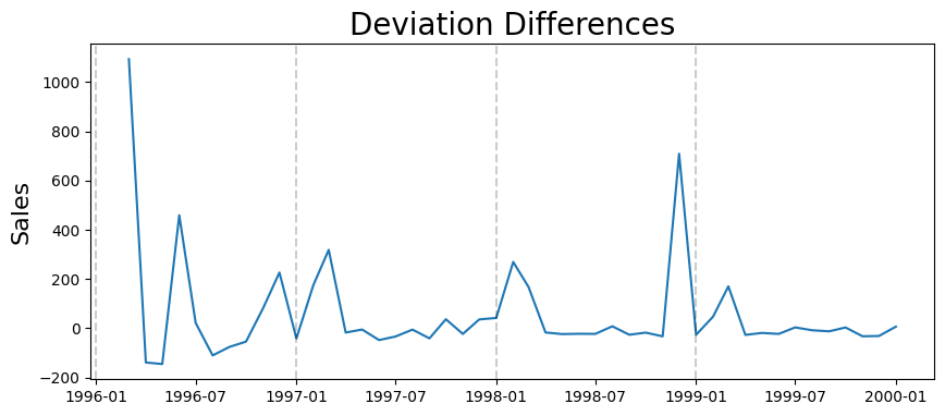
Attempt 1: Deviation Method#
plt.figure(figsize=(10,4))
plt.plot(lim_catfish_sales)
plt.title('Catfish Sales in 1000s of Pounds', fontsize=20)
plt.ylabel('Sales', fontsize=16)
for year in range(start_date.year,end_date.year):
    plt.axvline(pd.to_datetime(str(year)+'-01-01'), color='k', linestyle='--', alpha=0.2)

rolling_deviations = pd.Series(dtype=float, index = lim_catfish_sales.index)
for date in rolling_deviations.index:
    #get the window ending at this data point
    window = lim_catfish_sales.loc[:date]

    #get the deviation within this window
    rolling_deviations.loc[date] = window.std()
#get the difference in deviation between one time point and the next
diff_rolling_deviations = rolling_deviations.diff()
diff_rolling_deviations = diff_rolling_deviations.dropna()
plt.figure(figsize=(10,4))
plt.plot(diff_rolling_deviations)
plt.title('Deviation Differences', fontsize=20)
plt.ylabel('Sales', fontsize=16)
for year in range(start_date.year,end_date.year):
    plt.axvline(pd.to_datetime(str(year)+'-01-01'), color='k', linestyle='--', alpha=0.2)
Attempt 2: Seasonal Method#
month_deviations = lim_catfish_sales.groupby(lambda d: d.month).std()
plt.figure(figsize=(10,4))
plt.plot(month_deviations)
plt.title('Deviation by Month', fontsize=20)
plt.ylabel('Sales', fontsize=16)
Text(0, 0.5, 'Sales')
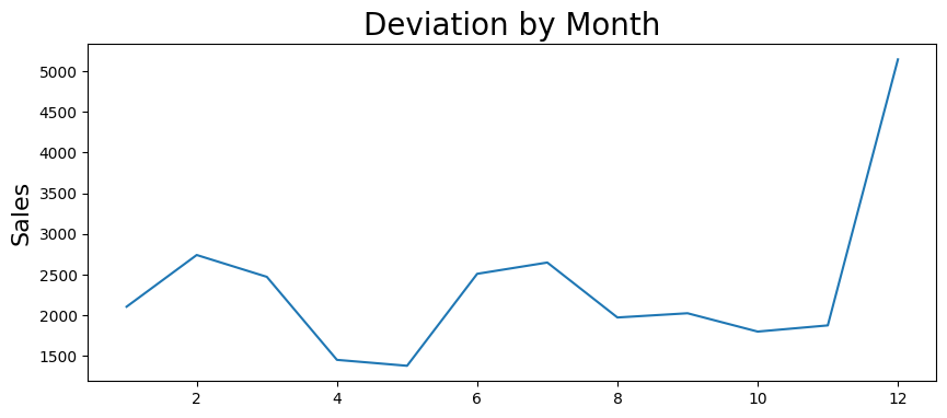
So, the anomaly occurs in a December#
december_data = lim_catfish_sales[lim_catfish_sales.index.month == 12]
december_data
Date
1996-12-01    16898
1997-12-01    18278
1998-12-01    10000
1999-12-01    22372
Name: Total, dtype: int64
min_dev = 9999999
curr_anomaly = None
for date in december_data.index:
    other_data = december_data[december_data.index != date]
    curr_dev = other_data.std()
    if curr_dev < min_dev:
        min_dev = curr_dev
        curr_anomaly = date
curr_anomaly
Timestamp('1998-12-01 00:00:00')
What to do about the anomaly?#
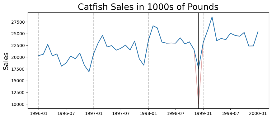
Simple Idea: use mean of other months#
adjusted_data = lim_catfish_sales.copy()
adjusted_data.loc[curr_anomaly] = december_data[(december_data.index != curr_anomaly) & (december_data.index < test_data.index[0])].mean()
plt.figure(figsize=(10,4))
plt.plot(lim_catfish_sales, color='firebrick', alpha=0.4)
plt.plot(adjusted_data)
plt.title('Catfish Sales in 1000s of Pounds', fontsize=20)
plt.ylabel('Sales', fontsize=16)
for year in range(start_date.year,end_date.year):
    plt.axvline(pd.to_datetime(str(year)+'-01-01'), color='k', linestyle='--', alpha=0.2)
plt.axvline(curr_anomaly, color='k', alpha=0.7)
<matplotlib.lines.Line2D at 0x7f10b1a3cd30>
Resulting Predictions#
train_end = datetime(1999,7,1)
test_end = datetime(2000,1,1)

test_data = adjusted_data[train_end + timedelta(days=1):test_end]
rolling_predictions = test_data.copy()
for train_end in test_data.index:
    train_data = adjusted_data[:train_end-timedelta(days=1)]
    model = SARIMAX(train_data, order=my_order, seasonal_order=my_seasonal_order)
    model_fit = model.fit()

    pred = model_fit.forecast()
    rolling_predictions[train_end] = pred
/home/ubuntu/Documents/Projects/STI_FX_Intervention/.venv/lib/python3.9/site-packages/statsmodels/tsa/statespace/sarimax.py:997: UserWarning: Non-stationary starting seasonal autoregressive Using zeros as starting parameters.
  warn('Non-stationary starting seasonal autoregressive'
 This problem is unconstrained.
/home/ubuntu/Documents/Projects/STI_FX_Intervention/.venv/lib/python3.9/site-packages/statsmodels/base/model.py:604: ConvergenceWarning: Maximum Likelihood optimization failed to converge. Check mle_retvals
  warnings.warn("Maximum Likelihood optimization failed to "
/home/ubuntu/Documents/Projects/STI_FX_Intervention/.venv/lib/python3.9/site-packages/statsmodels/tsa/statespace/sarimax.py:997: UserWarning: Non-stationary starting seasonal autoregressive Using zeros as starting parameters.
  warn('Non-stationary starting seasonal autoregressive'
/home/ubuntu/Documents/Projects/STI_FX_Intervention/.venv/lib/python3.9/site-packages/statsmodels/tsa/statespace/sarimax.py:1009: UserWarning: Non-invertible starting seasonal moving average Using zeros as starting parameters.
  warn('Non-invertible starting seasonal moving average'
RUNNING THE L-BFGS-B CODE

           * * *

Machine precision = 2.220D-16
 N =            3     M =           10

At X0         0 variables are exactly at the bounds

At iterate    0    f=  9.02989D+00    |proj g|=  1.39448D+00

At iterate    5    f=  8.65274D+00    |proj g|=  4.92136D-01

At iterate   10    f=  8.58895D+00    |proj g|=  1.41914D-02

At iterate   15    f=  8.58843D+00    |proj g|=  1.95742D-04

At iterate   20    f=  8.58841D+00    |proj g|=  8.25947D-03

At iterate   25    f=  8.58344D+00    |proj g|=  6.37140D-02

At iterate   30    f=  8.52923D+00    |proj g|=  6.24736D-03

At iterate   35    f=  8.52907D+00    |proj g|=  1.02194D-03

At iterate   40    f=  8.52895D+00    |proj g|=  1.88970D-03

At iterate   45    f=  8.52886D+00    |proj g|=  1.44991D-03

At iterate   50    f=  8.52884D+00    |proj g|=  6.55285D-04

           * * *

Tit   = total number of iterations
Tnf   = total number of function evaluations
Tnint = total number of segments explored during Cauchy searches
Skip  = number of BFGS updates skipped
Nact  = number of active bounds at final generalized Cauchy point
Projg = norm of the final projected gradient
F     = final function value

           * * *

   N    Tit     Tnf  Tnint  Skip  Nact     Projg        F
    3     50     68      1     0     0   6.553D-04   8.529D+00
  F =   8.5288391511597741

STOP: TOTAL NO. of ITERATIONS REACHED LIMIT
RUNNING THE L-BFGS-B CODE

           * * *

Machine precision = 2.220D-16
 N =            3     M =           10

At X0         0 variables are exactly at the bounds

At iterate    0    f=  9.01339D+00    |proj g|=  1.34785D+00

At iterate    5    f=  8.64177D+00    |proj g|=  4.38112D-01

At iterate   10    f=  8.59046D+00    |proj g|=  1.04906D-02

At iterate   15    f=  8.59022D+00    |proj g|=  2.14865D-04

At iterate   20    f=  8.59019D+00    |proj g|=  8.95238D-03

At iterate   25    f=  8.58544D+00    |proj g|=  6.49231D-02

At iterate   30    f=  8.52891D+00    |proj g|=  6.86211D-04

At iterate   35    f=  8.52880D+00    |proj g|=  3.23347D-03

At iterate   40    f=  8.52871D+00    |proj g|=  9.21060D-04
 This problem is unconstrained.

 Bad direction in the line search;
   refresh the lbfgs memory and restart the iteration.
           * * *

Tit   = total number of iterations
Tnf   = total number of function evaluations
Tnint = total number of segments explored during Cauchy searches
Skip  = number of BFGS updates skipped
Nact  = number of active bounds at final generalized Cauchy point
Projg = norm of the final projected gradient
F     = final function value

           * * *

   N    Tit     Tnf  Tnint  Skip  Nact     Projg        F
    3     44     74      2     0     0   8.741D-06   8.529D+00
  F =   8.5286758066920854

CONVERGENCE: NORM_OF_PROJECTED_GRADIENT_<=_PGTOL
RUNNING THE L-BFGS-B CODE

           * * *

Machine precision = 2.220D-16
 N =            3     M =           10

At X0         0 variables are exactly at the bounds

At iterate    0    f=  9.05490D+00    |proj g|=  1.51925D+00

At iterate    5    f=  8.64187D+00    |proj g|=  1.28743D-01

At iterate   10    f=  8.56327D+00    |proj g|=  2.44168D-02

At iterate   15    f=  8.56172D+00    |proj g|=  1.76571D-04

At iterate   20    f=  8.56171D+00    |proj g|=  1.23540D-03

At iterate   25    f=  8.56082D+00    |proj g|=  9.66500D-03

At iterate   30    f=  8.52254D+00    |proj g|=  1.02194D-02

At iterate   35    f=  8.52104D+00    |proj g|=  3.47220D-03

At iterate   40    f=  8.52086D+00    |proj g|=  5.34944D-03

At iterate   45    f=  8.52078D+00    |proj g|=  2.79134D-03

At iterate   50    f=  8.52075D+00    |proj g|=  7.59471D-04

           * * *

Tit   = total number of iterations
Tnf   = total number of function evaluations
Tnint = total number of segments explored during Cauchy searches
Skip  = number of BFGS updates skipped
Nact  = number of active bounds at final generalized Cauchy point
Projg = norm of the final projected gradient
F     = final function value

           * * *

   N    Tit     Tnf  Tnint  Skip  Nact     Projg        F
    3     50     62      1     0     0   7.595D-04   8.521D+00
  F =   8.5207537625163301

STOP: TOTAL NO. of ITERATIONS REACHED LIMIT
/home/ubuntu/Documents/Projects/STI_FX_Intervention/.venv/lib/python3.9/site-packages/statsmodels/tsa/statespace/sarimax.py:997: UserWarning: Non-stationary starting seasonal autoregressive Using zeros as starting parameters.
  warn('Non-stationary starting seasonal autoregressive'
/home/ubuntu/Documents/Projects/STI_FX_Intervention/.venv/lib/python3.9/site-packages/statsmodels/tsa/statespace/sarimax.py:1009: UserWarning: Non-invertible starting seasonal moving average Using zeros as starting parameters.
  warn('Non-invertible starting seasonal moving average'
 This problem is unconstrained.
/home/ubuntu/Documents/Projects/STI_FX_Intervention/.venv/lib/python3.9/site-packages/statsmodels/base/model.py:604: ConvergenceWarning: Maximum Likelihood optimization failed to converge. Check mle_retvals
  warnings.warn("Maximum Likelihood optimization failed to "
/home/ubuntu/Documents/Projects/STI_FX_Intervention/.venv/lib/python3.9/site-packages/statsmodels/tsa/statespace/sarimax.py:997: UserWarning: Non-stationary starting seasonal autoregressive Using zeros as starting parameters.
  warn('Non-stationary starting seasonal autoregressive'
/home/ubuntu/Documents/Projects/STI_FX_Intervention/.venv/lib/python3.9/site-packages/statsmodels/tsa/statespace/sarimax.py:1009: UserWarning: Non-invertible starting seasonal moving average Using zeros as starting parameters.
  warn('Non-invertible starting seasonal moving average'
 This problem is unconstrained.
RUNNING THE L-BFGS-B CODE

           * * *

Machine precision = 2.220D-16
 N =            3     M =           10

At X0         0 variables are exactly at the bounds

At iterate    0    f=  9.09568D+00    |proj g|=  1.65700D+00

At iterate    5    f=  8.69211D+00    |proj g|=  4.53682D-01

At iterate   10    f=  8.54756D+00    |proj g|=  3.40350D-02

At iterate   15    f=  8.54083D+00    |proj g|=  3.33430D-03

At iterate   20    f=  8.54082D+00    |proj g|=  1.58057D-04

At iterate   25    f=  8.54078D+00    |proj g|=  1.06184D-02

At iterate   30    f=  8.53674D+00    |proj g|=  1.18313D-01

At iterate   35    f=  8.51481D+00    |proj g|=  3.12128D-03

At iterate   40    f=  8.51245D+00    |proj g|=  3.27935D-03

At iterate   45    f=  8.51183D+00    |proj g|=  4.67688D-03

At iterate   50    f=  8.51160D+00    |proj g|=  6.58486D-03

           * * *

Tit   = total number of iterations
Tnf   = total number of function evaluations
Tnint = total number of segments explored during Cauchy searches
Skip  = number of BFGS updates skipped
Nact  = number of active bounds at final generalized Cauchy point
Projg = norm of the final projected gradient
F     = final function value

           * * *

   N    Tit     Tnf  Tnint  Skip  Nact     Projg        F
    3     50     58      1     0     0   6.585D-03   8.512D+00
  F =   8.5116027468333648

STOP: TOTAL NO. of ITERATIONS REACHED LIMIT
RUNNING THE L-BFGS-B CODE

           * * *

Machine precision = 2.220D-16
 N =            3     M =           10

At X0         0 variables are exactly at the bounds

At iterate    0    f=  9.11292D+00    |proj g|=  1.65876D+00
/home/ubuntu/Documents/Projects/STI_FX_Intervention/.venv/lib/python3.9/site-packages/statsmodels/base/model.py:604: ConvergenceWarning: Maximum Likelihood optimization failed to converge. Check mle_retvals
  warnings.warn("Maximum Likelihood optimization failed to "
/home/ubuntu/Documents/Projects/STI_FX_Intervention/.venv/lib/python3.9/site-packages/statsmodels/tsa/statespace/sarimax.py:997: UserWarning: Non-stationary starting seasonal autoregressive Using zeros as starting parameters.
  warn('Non-stationary starting seasonal autoregressive'
/home/ubuntu/Documents/Projects/STI_FX_Intervention/.venv/lib/python3.9/site-packages/statsmodels/tsa/statespace/sarimax.py:1009: UserWarning: Non-invertible starting seasonal moving average Using zeros as starting parameters.
  warn('Non-invertible starting seasonal moving average'
 This problem is unconstrained.
At iterate    5    f=  8.69850D+00    |proj g|=  5.10951D-01

At iterate   10    f=  8.54796D+00    |proj g|=  3.33515D-02

At iterate   15    f=  8.54222D+00    |proj g|=  3.24499D-03

At iterate   20    f=  8.54169D+00    |proj g|=  9.91802D-04

At iterate   25    f=  8.50994D+00    |proj g|=  3.59922D-02

At iterate   30    f=  8.50916D+00    |proj g|=  3.60959D-03

At iterate   35    f=  8.50902D+00    |proj g|=  2.80777D-03

At iterate   40    f=  8.50899D+00    |proj g|=  2.60936D-03

At iterate   45    f=  8.50896D+00    |proj g|=  1.05368D-03
  ys=-9.422E-07  -gs= 2.177E-06 BFGS update SKIPPED

At iterate   50    f=  8.50895D+00    |proj g|=  1.44994D-03

           * * *

Tit   = total number of iterations
Tnf   = total number of function evaluations
Tnint = total number of segments explored during Cauchy searches
Skip  = number of BFGS updates skipped
Nact  = number of active bounds at final generalized Cauchy point
Projg = norm of the final projected gradient
F     = final function value

           * * *

   N    Tit     Tnf  Tnint  Skip  Nact     Projg        F
    3     50     78      1     1     0   1.450D-03   8.509D+00
  F =   8.5089495859676330

STOP: TOTAL NO. of ITERATIONS REACHED LIMIT
RUNNING THE L-BFGS-B CODE

           * * *

Machine precision = 2.220D-16
 N =            3     M =           10

At X0         0 variables are exactly at the bounds

At iterate    0    f=  8.72720D+00    |proj g|=  5.58769D-01

At iterate    5    f=  8.61908D+00    |proj g|=  1.33323D-01

At iterate   10    f=  8.59171D+00    |proj g|=  6.72396D-03

At iterate   15    f=  8.59153D+00    |proj g|=  3.52489D-04

At iterate   20    f=  8.59137D+00    |proj g|=  4.54451D-03
/home/ubuntu/Documents/Projects/STI_FX_Intervention/.venv/lib/python3.9/site-packages/statsmodels/base/model.py:604: ConvergenceWarning: Maximum Likelihood optimization failed to converge. Check mle_retvals
  warnings.warn("Maximum Likelihood optimization failed to "
/home/ubuntu/Documents/Projects/STI_FX_Intervention/.venv/lib/python3.9/site-packages/statsmodels/tsa/statespace/sarimax.py:1009: UserWarning: Non-invertible starting seasonal moving average Using zeros as starting parameters.
  warn('Non-invertible starting seasonal moving average'
 This problem is unconstrained.
At iterate   25    f=  8.56045D+00    |proj g|=  5.88962D-02

At iterate   30    f=  8.51572D+00    |proj g|=  9.39532D-04

At iterate   35    f=  8.51560D+00    |proj g|=  4.53458D-03

At iterate   40    f=  8.51555D+00    |proj g|=  1.48086D-04

At iterate   45    f=  8.51550D+00    |proj g|=  1.45504D-03

At iterate   50    f=  8.51549D+00    |proj g|=  5.86388D-04

           * * *

Tit   = total number of iterations
Tnf   = total number of function evaluations
Tnint = total number of segments explored during Cauchy searches
Skip  = number of BFGS updates skipped
Nact  = number of active bounds at final generalized Cauchy point
Projg = norm of the final projected gradient
F     = final function value

           * * *

   N    Tit     Tnf  Tnint  Skip  Nact     Projg        F
    3     50     85      1     0     0   5.864D-04   8.515D+00
  F =   8.5154939893926826

STOP: TOTAL NO. of ITERATIONS REACHED LIMIT
/home/ubuntu/Documents/Projects/STI_FX_Intervention/.venv/lib/python3.9/site-packages/statsmodels/base/model.py:604: ConvergenceWarning: Maximum Likelihood optimization failed to converge. Check mle_retvals
  warnings.warn("Maximum Likelihood optimization failed to "
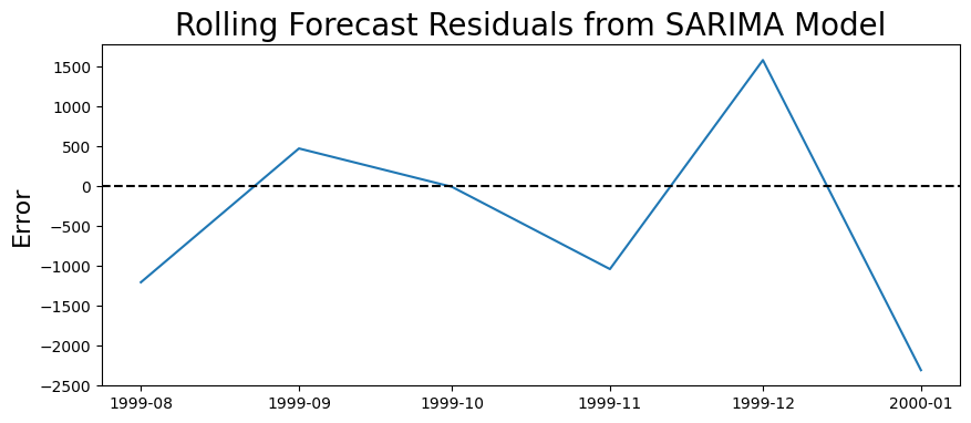
rolling_residuals = test_data - rolling_predictions
plt.figure(figsize=(10,4))
plt.plot(rolling_residuals)
plt.axhline(0, linestyle='--', color='k')
plt.title('Rolling Forecast Residuals from SARIMA Model', fontsize=20)
plt.ylabel('Error', fontsize=16)
Text(0, 0.5, 'Error')
plt.figure(figsize=(10,4))

plt.plot(lim_catfish_sales)
plt.plot(rolling_predictions)

plt.legend(('Data', 'Predictions'), fontsize=16)

plt.title('Catfish Sales in 1000s of Pounds', fontsize=20)
plt.ylabel('Production', fontsize=16)
for year in range(start_date.year,end_date.year):
    plt.axvline(pd.to_datetime(str(year)+'-01-01'), color='k', linestyle='--', alpha=0.2)
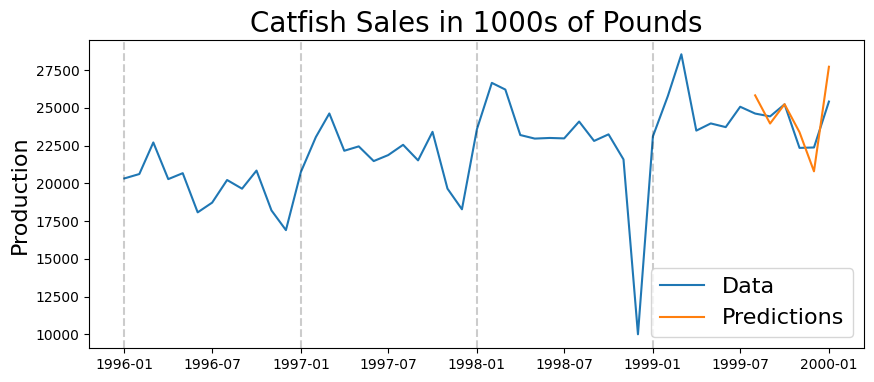
print('Mean Absolute Percent Error:', round(np.mean(abs(rolling_residuals/test_data)),4))
Mean Absolute Percent Error: 0.0461
print('Root Mean Squared Error:', np.sqrt(np.mean(rolling_residuals**2)))
Root Mean Squared Error: 1327.4209125685188

